About
This documentation aims to help reproduce the experiments described in the paper Querying Wikidata: Comparing SPARQL, Relational and Graph Databases (by Daniel Hernández, Aidan Hogan, Cristian Riveros, Carlos Rojas and Enzo Zerega).
These pages were generated using Jekyll from the source available in the repository wquery-docs. Also, this documentation is accessible on the following URLs:
- http://users.dcc.uchile.cl/~dhernand/wquery/ (this website).
- https://dx.doi.org/10.6084/m9.figshare.3219217.v3 (DOI pointing this website).
The documentation is laid out as follows:
- License: details of licencing for original and third-party material
- Dataset and code: links to download (mirrored) dataset and necessary code
- Queries: details of queries generated for the benchmark
- Experimental Setting: details of the hardware/software setting used in the paper
- Repeating the experiments: step-by-step guide for repeating the experiments presented
- Results: raw and supplementary results supporting the paper
License
All our code and documentation is published under the Creative Commons CC-BY License. The Wikidata dump is published under Creative Commons CC0 License.
All of the engines used in these experiments are distributed under open licenses. PostgreSQL uses the PostgreSQL License, Virtuoso Opensource uses the GPLv2 Licence, Blazegraph uses the GPLv2 License licence and Neo4j Community Edition uses the GPLv3 License.
Dataset and code
To reproduce these experiments, it is necessary to download and install the database engines and the following resources:
Code and results (https://bitbucket.org/danielhz/wikidata-experiments). The code required to repeat these experiments is published in this repository. Also, parameters to generate queries and results of experiments are published in this repository.
Dataset (https://dx.doi.org/10.6084/m9.figshare.3208498.v1). All experiments are done using the dump of Wikidata published on January 4th, 2016. The original dump was downloaded from the dumps folder published by the Wikimedia Foundation. However, the contents in this folder are frequently updated and old dumps are discarded. Thus, in the interest of sustainability, we published the dump used on Figshare.
Queries
The experiments presented in the paper consider two groups of queries: atomic queries that are based on quins and more complex queries that are structured as snowflakes of various depth.
Atomic quin queries
Quin queries have the following components:
?x0Item (s).?x1Claim property (p).?x2Property value (o).?x3Qualifier property (q).?x4Qualifier value (v).
We create different atomic queries using different patterns where various
positions are either variable or constant: we use bitmasks to represent
these patterns where, for example the bitmask 01110 indicates that
p, o, q are variables and s, v are constants.
For each bitmask a file with 300 queries is generated, where each query is a quin
following that bitmask. For example, the following quin
is in the CSV file query_parameters/quins/quins_01110.csv of the repository
(that corresponds to the bitmask 01110).
?x0 P2239 Q21402571 P636 ?x4
Note: Each such query is generated from the data and thus will produce non-empty results.
Note: The variables ?x1 to ?x3 are replaced with constants because
the bitmask contains a 1 in these positions.
Note: The property value and the qualifier value are value items (not datatype values).
Each quin will then be converted into a “concrete query” for the particular
setting, where we will momentarily present examples for the previous 01110 quin.
Note: If the qualifier property or the qualifier value are not specified,
then a left outer join is used. Thus, the operators OPTIONAL,
OPTIONAL MATCH and LEFT OUTER JOIN are used in the SPARQL, Cypher and
SQL implementations, respectively.
SPARQL (n-ary relations)
PREFIX wd: <http://www.wikidata.org/entity/>
PREFIX p: <http://www.wikidata.org/prop/>
PREFIX ps: <http://www.wikidata.org/prop/statement/>
SELECT ?s ?qo
WHERE { ?s p:P2239 ?c . ?c ps:P2239 wd:Q21402571 ; p:P636 ?qo . }
LIMIT 10000
SPARQL (named graphs)
PREFIX wd: <http://www.wikidata.org/entity/>
PREFIX p: <http://www.wikidata.org/prop/>
SELECT ?s ?qo
WHERE { GRAPH ?c { ?s p:P2239 wd:Q21402571 . ?c p:P636 ?qo } .
        FILTER (?s != ?c) }
LIMIT 10000
SPARQL (singleton properties)
PREFIX wd: <http://www.wikidata.org/entity/>
PREFIX p: <http://www.wikidata.org/prop/>
PREFIX rdf: <http://www.w3.org/1999/02/22-rdf-syntax-ns#>
SELECT ?s ?qo
WHERE { ?s ?c wd:Q21402571 .
        ?c rdf:singletonPropertyOf p:P2239 ; p:P636 ?qo . }
LIMIT 10000
SPARQL (standard reification)
PREFIX wd: <http://www.wikidata.org/entity/>
PREFIX p: <http://www.wikidata.org/prop/>
PREFIX rdf: <http://www.w3.org/1999/02/22-rdf-syntax-ns#>
SELECT ?s ?qo
WHERE { ?c rdf:subject ?s ;
           rdf:predicate p:P2239 ;
           rdf:object wd:Q21402571 ;
           p:P636 ?qo . }
LIMIT 10000
Cypher
MATCH (s:Item)-[:PROP_FROM]->(c:Claim)-[:PROP_TO]->(o),
      (c)-[:PROPERTY]->(p:Property),
      (c)-[:QUAL_FROM]->(qn:Qualifier)-[:QUAL_TO]->(q),
      (qn)-[:PROPERTY]->(qp:Property)
WHERE p.id='P2239' AND
      o.id='Q21402571' AND
      qp.id='P636'
RETURN s.id, q.id
LIMIT 10000;
SQL
SELECT
  claims.entity_id,
  qualifiers.datavalue_entity
FROM
  claims,
  qualifiers
WHERE
  qualifiers.claim_id = claims.id AND
  claims.property = 'P2239' AND
  claims.datavalue_entity = 'Q21402571' AND
  qualifiers.property = 'P636'
Snowflake (depth-*) queries
Snowflake queries are generated using a list of nodes (codified in JSON).
Each node represents an item (identified with the attribute entity_id)
of such nodes. For each node, a set of claims is selected. Each claim is
codified with a pair [P,X], where P is the claim property and X is a
item value id, a 0 (the item value of the claim is not projected in the
solution) or a 1 (the item value of the claim is projected in the solution).
Also, the attribute property codifies the property that joins nodes in the
snowflake. For example, the following is a raw snowflake pattern:
[{"entity_id":"Q6260140",
  "claims":[["P102",0],["P735","Q4925477"],["P31",0]],
  "property":"P27"},
 {"entity_id":"Q30"
  "claims":[["P1792",1]],
  "property":"P530"},
 {"entity_id":"Q408",
  "claims":[["P1343",1],["P1792",1]]}]
The snowflake parameters are stored in the folder
query_parameters/paths of the code repository. To generate these
parameters we first generate the tables containing tuples with items
that are connected and that have at least an out-degree of 5 to
other items. The raw tables are generated with the SQL scripts in
the folder wikidata-experiments/sql/parameters_2. Then we run the
following command:
cd wikidata-experiments/sql/parameters_2
./generate_path.rb 1 500
./generate_path.rb 2 500
In the following, we give examples of the concrete queries generated from the raw snowflake presented above.
SPARQL (n-ary relations)
PREFIX wd: <http://www.wikidata.org/entity/>
PREFIX p: <http://www.wikidata.org/prop/>
PREFIX ps: <http://www.wikidata.org/prop/statement/>
PREFIX wikibase: <http://wikiba.se/ontology-beta#>
SELECT ?x0 ?x1 ?x1y0 ?x2 ?x2y0 ?x2y1
WHERE {
  ?x0 p:P102 ?claim_x0y0 .
  ?claim_x0y0 ps:P102 ?x0y0 .
  ?x0 p:P735 ?claim_x0y1 .
  ?claim_x0y1 ps:P735 wd:Q4925477 .
  ?x0 p:P31 ?claim_x0y2 .
  ?claim_x0y2 ps:P31 ?x0y2 .
  ?x0 p:P27 ?claim_x0 .
  ?claim_x0 ps:P27 ?x1 .
  ?x1 p:P1792 ?claim_x1y0 .
  ?claim_x1y0 ps:P1792 ?x1y0 .
  ?x1 p:P530 ?claim_x1 .
  ?claim_x1 ps:P530 ?x2 .
  ?x2 p:P1343 ?claim_x2y0 .
  ?claim_x2y0 ps:P1343 ?x2y0 .
  ?x2 p:P1792 ?claim_x2y1 .
  ?claim_x2y1 ps:P1792 ?x2y1 . }
LIMIT 10000
SPARQL (named graphs)
PREFIX wd: <http://www.wikidata.org/entity/>
PREFIX p: <http://www.wikidata.org/prop/>
SELECT ?x0 ?x1 ?x1y0 ?x2 ?x2y0 ?x2y1
WHERE {
  GRAPH ?claim_x0y0 { ?x0 p:P102 ?x0y0 } .
  GRAPH ?claim_x0y1 { ?x0 p:P735 wd:Q4925477 } .
  GRAPH ?claim_x0y2 { ?x0 p:P31 ?x0y2 } .
  GRAPH ?claim_x0 { ?x0 p:P27 ?x1 } .
  GRAPH ?claim_x1y0 { ?x1 p:P1792 ?x1y0 } .
  GRAPH ?claim_x1 { ?x1 p:P530 ?x2 } .
  GRAPH ?claim_x2y0 { ?x2 p:P1343 ?x2y0 } .
  GRAPH ?claim_x2y1 { ?x2 p:P1792 ?x2y1 } . }
LIMIT 10000
SPARQL (singleton properties)
PREFIX wd: <http://www.wikidata.org/entity/>
PREFIX rdf: <http://www.w3.org/1999/02/22-rdf-syntax-ns#>
PREFIX p: <http://www.wikidata.org/prop/>
SELECT ?x0 ?x1 ?x1y0 ?x2 ?x2y0 ?x2y1
WHERE {
  ?x0 ?claim_x0y0 ?x0y0 . ?claim_x0y0 rdf:singletonPropertyOf p:P102 .
  ?x0 ?claim_x0y1 wd:Q4925477 . ?claim_x0y1 rdf:singletonPropertyOf p:P735 .
  ?x0 ?claim_x0y2 ?x0y2 . ?claim_x0y2 rdf:singletonPropertyOf p:P31 .
  ?x0 ?claim_x0 ?x1 . ?claim_x0 rdf:singletonPropertyOf p:P27 .
  ?x1 ?claim_x1y0 ?x1y0 . ?claim_x1y0 rdf:singletonPropertyOf p:P1792 .
  ?x1 ?claim_x1 ?x2 . ?claim_x1 rdf:singletonPropertyOf p:P530 .
  ?x2 ?claim_x2y0 ?x2y0 . ?claim_x2y0 rdf:singletonPropertyOf p:P1343 .
  ?x2 ?claim_x2y1 ?x2y1 . ?claim_x2y1 rdf:singletonPropertyOf p:P1792 . }
LIMIT 10000
SPARQL (standard reification)
PREFIX wd: <http://www.wikidata.org/entity/>
PREFIX p: <http://www.wikidata.org/prop/>
PREFIX rdf: <http://www.w3.org/1999/02/22-rdf-syntax-ns#>
SELECT ?x0 ?x1 ?x1y0 ?x2 ?x2y0 ?x2y1
WHERE {
  ?claim_x0y0 rdf:subject ?x0 .
  ?claim_x0y0 rdf:predicate p:P102 .
  ?claim_x0y0 rdf:object ?x0y0 .
  ?claim_x0y1 rdf:subject ?x0 .
  ?claim_x0y1 rdf:predicate p:P735 .
  ?claim_x0y1 rdf:object wd:Q4925477 .
  ?claim_x0y2 rdf:subject ?x0 .
  ?claim_x0y2 rdf:predicate p:P31 .
  ?claim_x0y2 rdf:object ?x0y2 .
  ?claim_x0 rdf:subject ?x0 .
  ?claim_x0 rdf:predicate p:P27 .
  ?claim_x0 rdf:object ?x1 .
  ?claim_x1y0 rdf:subject ?x1 .
  ?claim_x1y0 rdf:predicate p:P1792 .
  ?claim_x1y0 rdf:object ?x1y0 .
  ?claim_x1 rdf:subject ?x1 .
  ?claim_x1 rdf:predicate p:P530 .
  ?claim_x1 rdf:object ?x2 .
  ?claim_x2y0 rdf:subject ?x2 .
  ?claim_x2y0 rdf:predicate p:P1343 .
  ?claim_x2y0 rdf:object ?x2y0 .
  ?claim_x2y1 rdf:subject ?x2 .
  ?claim_x2y1 rdf:predicate p:P1792 .
  ?claim_x2y1 rdf:object ?x2y1 . }
LIMIT 10000
Cypher
MATCH (x0:Item)-[:PROP_FROM]->(c0:Claim)-[:PROP_TO]->(x1:Item),
      (c0)-[:PROPERTY]->(:Property {id:"P27"}),
      (x0)-[:PROP_FROM]->(cx0y0:Claim)-[:PROP_TO]->(x0y0:Item),
      (cx0y0)-[:PROPERTY]->(:Property {id:"P102"}),
      (x0)-[:PROP_FROM]->(cx0y1:Claim)-[:PROP_TO]->(x0y1:Item {id:"Q4925477"}),
      (cx0y1)-[:PROPERTY]->(:Property {id:"P735"}),
      (x0)-[:PROP_FROM]->(cx0y2:Claim)-[:PROP_TO]->(x0y2:Item),
      (cx0y2)-[:PROPERTY]->(:Property {id:"P31"}),
      (x1:Item)-[:PROP_FROM]->(c1:Claim)-[:PROP_TO]->(x2:Item),
      (c1)-[:PROPERTY]->(:Property {id:"P530"}),
      (x1)-[:PROP_FROM]->(cx1y0:Claim)-[:PROP_TO]->(x1y0:Item),
      (cx1y0)-[:PROPERTY]->(:Property {id:"P1792"}),
      (x2)-[:PROP_FROM]->(cx2y0:Claim)-[:PROP_TO]->(x2y0:Item),
      (cx2y0)-[:PROPERTY]->(:Property {id:"P1343"}),
      (x2)-[:PROP_FROM]->(cx2y1:Claim)-[:PROP_TO]->(x2y1:Item),
      (cx2y1)-[:PROPERTY]->(:Property {id:"P1792"})
RETURN x0.id x1.id x1y0.id x2.id x2y0.id x2y1.id
LIMIT 10000;
SQL
SELECT
  c0.entity_id,
  c1.entity_id,
  x1y0.datavalue_entity,
  c2.entity_id,
  x2y0.datavalue_entity,
  x2y1.datavalue_entity
FROM
  claims AS c0,
  claims AS c1,
  claims AS cx0y0,
  claims AS cx0y1,
  claims AS cx0y2,
  claims AS cx1y0,
  claims AS cx2y0,
  claims AS cx2y1
WHERE
  c0.datavalue_entity = c1.entity_id AND
  c0.property = 'P27' AND
  c0.datavalue_entity = cx0y0.entity_id AND
  cx0y0.property = 'P102' AND
  c0.datavalue_entity = cx0y1.entity_id AND
  cx0y1.property = 'P735' AND
  cx0y1.datavalue_entity = 'Q4925477' AND
  c0.datavalue_entity = cx0y2.entity_id AND
  cx0y2.property = 'P31' AND
  c1.datavalue_entity = c2.entity_id AND
  c1.property = 'P530' AND
  c1.datavalue_entity = cx1y0.entity_id AND
  cx1y0.property = 'P1792' AND
  c2.datavalue_entity = cx2y0.entity_id AND
  cx2y0.property = 'P1343' AND
  c2.datavalue_entity = cx2y1.entity_id AND
  cx2y0.property = 'P1792'
Experimental settings
Here we describe the specific setting in which we ran experiments for the paper.
Machine: All experiments were run on a single machine with 2× Intel Xeon Six Core E5-2609 V3 CPUs, 32GB of RAM, and 2× 1TB Seagate 7200 RPM 32MB Cache SATA hard-disks in a RAID-1 configuration.
System: All experiments where run on a Debian 7 system using Ruby 2.3,
Python 2 and Bash scripts. The partition mounted in / (which has only 55GB)
is not enough for the data used. Thus, when necessary we use the partition
mounted in /home (which has 1.7TB) for the data.
Timeouts: We assumed a server-side timeout of 60 seconds per query.
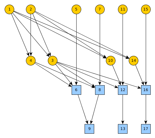
Repeating the experiments
The list below enumerates the tasks required to perform the experiments. The figure below shows what tasks can be done in parallel. Tasks that are enclosed in squares should be done on a dedicated machine (without other processes running in the background). We recommend executing these tasks with GNU Screen.
Note: We assume that distributions compatible with Ruby 2.3, Python 2 and Java 7.0 have been installed.
Note: In the documentation of these tasks, shell variables (e.g. $USER,
$WD_HOME) will be used. You will have to set these shell variables according
to your own settings.
Note: All experiments will be run by a user identified as $USER whose
home is $USER_HOME. Also, $USER should be in the sudo group.
Diagram of tasks
List of tasks
- Download the code.
- Download the dataset.
- Generate the raw queries
- Translate the raw data to RDF.
- Configure Virtuoso
- Load the data into Virtuoso.
- Configure Blazegraph
- Load the data into Blazegraph.
- Generate SPARQL queries and run experiments in Virtuoso and Blazegraph
- Translate the raw data to relational model.
- Configure PostgreSQL.
- Load the data into PostgreSQL.
- Generate SQL queries and run experiments in PostgreSQL.
- Translate the data to the Neo4j data model.
- Configure Neo4j.
- Load the data in Neo4j.
- Run experiments in Neo4j.
1. Download the code
The code is tracked in a git repository. You can get the code with the following command:
git clone https://bitbucket.org/danielhz/wikidata-experiments.git
In what follows, we refer to the folder created by git as $WD_HOME.
2. Download the dataset
You can download the dataset with the following command:
wget https://dx.doi.org/10.6084/m9.figshare.3208498.v1
In what follows, we refer to the file created by wget as $DATASET.
3. Generate the raw queries
The next step is to generate raw queries from the data. These queries will later be converted to concrete queries in SPARQL, SQL and Cypher. Please see the Queries section for more details.
To generate the atomic quin queries, execute:
cd $WD_HOME
bin/generate_quins.rb
To generate the snowflake queries at depth 1 and 2, execute:
cd wikidata-experiments/sql/parameters_2
./generate_path.rb 1 500
./generate_path.rb 2 500
4. Translate the raw data to RDF
Before translating the data to the RDF model, we need to split it into several smaller files (the translation process leaks memory so splitting it ensures that the process ends without getting an out memory exception). Translating each small file is done by an independent process.
The commands below prepare the dataset. We assume that $DATASET is
the path to the dataset, $RDF is the folder where we store
the RDF versions of the dataset and $WD_HOME is the folder of the
code.
cd $RDF
bunzip2 -c $DATASET | split -d -a 3 -C 100000000
rename '/$/.json/' x*
gzip x*.json
cd $WD_HOME
translation/translate_all.rb $RDF
After running the above commands, the $RDF folder will contain several JSON
files (e.g., x000.json.gz, x001.json.gz, where x001 indicates a file-part).
For each of these JSON files, four NQuads files are created, one for each schema.
They are named using the keywords naryrel (n-ary relations), ngraphs (named graphs),
sgprop (singleton properties) and stdreif (standard reification).
For example, the file-part x000.json.gz is translated into
the files x000-naryrel.nq.gz, x000-ngraphs.nq.gz,
x000-sgprop.nq.gz and x000-stdreif.nq.gz.
Note: We use the environment name $SCHEMA for the current schema in RDF experiments,
which can be one of naryrel, ngraphs, sgprop or stdreif.
5. Configure Virtuoso
We used Virtuoso Open Source Edition (7.2.3-dev.3215-pthreads), compiled from the source.
For each $SCHEMA there is a directory
$WD_HOME/dbfiles/virtuoso/db-$SCHEMA-1. Initially, this folder contains
only the file virtuoso.ini inside.
By default, Virtuoso stores the data in a folder in the / partition
(that does not have enough space in our setting). Inside this folder
we create a symbolic link to the database folder of each $SCHEMA.
$ cd /usr/local/virtuoso-opensource/var/lib/virtuoso/
$ ln -s $WD_HOME/dbfiles/virtuoso/db-$SCHEMA-1 db-$SCHEMA-1
The following variables are set in virtuoso.ini file of each $SCHEMA.
NumberOfBuffers            = 2720000
MaxDirtyBuffers            = 2000000
MaxQueryCostEstimationTime = 0
MaxQueryExecutionTime      = 60
The values for the properties NumberOfBuffers and MaxDirtyBuffers are
recommended in the configuration file for a machine with 32GB of memory
(as our machine has).
The property MaxQueryCostEstimationTime indicates the maximum estimated time
for a query. If the engine estimates that a query will take longer than this
value, then it will not try to evaluate it. We set this property to 0, which
means that no estimation limits are applied; i.e., Virtuoso will attempt
to evaluate all queries.
Finally, the MaxQueryExecutionTime is the timeout for query execution.
Queries that exceed this timeout are aborted at runtime.
Note: In Virtuoso the default dataset is always assumed to be the union of all named graphs. Thus, no specific configuration is needed to get this behavior with the named graphs schema.
6. Load the data into Virtuoso
To load the data it is assumed that Virtuoso is installed into
/usr/local/virtuoso-opensource/var/lib/virtuoso/ ($VIRTUOSO_HOME
in what follows). Also, we assume that the file $VIRTUOSO_CONFIG
contains the configuration details for Virtuoso and that
$DB_NARYREL, $DB_NAGRAPHS, $DB_SGPROP and
$DB_STDREIF are empty directories.
We load the data into Virtuoso with the following commands:
cd $DB_NARYREL
ln -s $VIRTUOSO_CONFIG virtuoso.ini
mkdir wikidata
cd $DB_NGRAPHS
ln -s $VIRTUOSO_CONFIG virtuoso.ini
mkdir wikidata
cd $DB_SGPROP
ln -s $VIRTUOSO_CONFIG virtuoso.ini
mkdir wikidata
cd $DB_STDREIF
ln -s $VIRTUOSO_CONFIG virtuoso.ini
mkdir wikidata
cd $WD_HOME/loading/virtuoso/
./load_data.rb
7. Configure Blazegraph
We used Blazegraph 2.1.0 Community Edition with Java 7. We use the Java implementation distributed by ORACLE (Java(TM) SE Runtime Environment build 1.7.0_80-b15).
Some parameters are added to the command line to improve the resource usage of the process. We set the JVM heap to 6GB and we use the G1 garbage collector of the Hostpot JVM (The JVM provides several garbage collectors): the documentation recommends these parameters.
We use the exec primitive in a Ruby script to start Blazegraph
with the following parameters:
exec(['java', 'blazegraph'],
  '-Xmx6g',
  '-XX:+UseG1GC',
  '-Djetty.overrideWebXml=override.xml',
  '-Dbigdata.propertyFile=server.properties',
  '-jar',
  'blazegraph.jar')
The override.xml file define a timeout of 60 seconds for query execution
and the server.properties file defines the parameters of the execution and
properties of the storage. Both configuration files can be found in the
code repository
of our experiments.
Note: In Blazegraph the default dataset is always assumed to be the union of all named graphs. Thus, no specific configuration is needed to get this behavior with the named graphs schema.
8. Load the data into Blazegraph
Blazegraph provides several data storage options. We use triple stores for experiments with n-ary relations, singleton properties and standard reification. For named graphs, we use a quad store.
The configuration for each backend is in the files
$WD_HOME/dbfiles/blazegraph/triples.properties and
$WD_HOME/dbfiles/blazegraph/quads.properties, respectively.
9. Generate SPARQL queries and run experiments in Virtuoso and Blazegraph
The SPARQL benchmarks use a configuration file containing the parameters that are necessary to run each experiment. The procedures to run experiments in Virtuoso and Blazegraph are the same. Thus, the following commands show how experiments are run in both engines.
$ cd $WD_HOME
$ bin/run_quins_benchmark config/virtuoso.rb
$ bin/run_quins_benchmark config/blazegraph.rb
$ bin/run_paths_benchmark config/paths_virtuoso.rb
$ bin/run_paths_benchmark config/paths_blazegraph.rb
Results for the quin benchmark are published in the folder results/quins of
the repository. Similarly, the results for the experiments with snowflake
structure are published in the folder results/paths.
After running these scripts, a CSV file is created for each set of queries.
Each file-name contains a reference to the engine, representation and query-set.
For example, the file results_blazegraph_onaryrel_01110.csv corresponds
to the results obtained for atomic quin queries with bitmask key 01110
using the Blazegraph engine for the n-ary relations representation.
The following is an example line from the results:
naryrel,path_1,0,11.50489629,125,200
We see, respectively, the RDF schema, the type of query run, the ID of the specific query, the time taken, the number of results returned (if not timeout) and a 200 code indicating success (or timeout if a timeout is reached).
10. Translate the data to the relational model
The following commands generate six CSV files from the Wikidata dump
in the folder csv (relative to the script). We assume that
$DATASET is the file containing the original dataset.
cd $WD_HOME/postgresql-experiment-scripts/loading-data/
bunzip2 -c $DATASET > dump.json
ruby migrador.rb
11. Configure PostgreSQL
We used PostgreSQL 9.1.20 with the folowing variables set in the
postgres.conf file:
default_statistics_target     = 100
maintenance_work_mem          = 1920MB
shared_buffers                = 7680MB
wal_buffers                   = 16MB
effective_cache_size          = 22GB
work_mem                      = 160MB
default_transaction_isolation = 'read uncommitted'
statement_timeout             = 60010
We used pgtune: a script to
automatically generate a configuration for PostgresSQL on our server.
This script is based on the recommendations in the
PostgresSQL Wiki
and sets the values of properties maintenance_work_mem,
shared_buffers and effective_cache_size. We also set
the lowest level of isolation whereby transactions are isolated just enough
to ensure that physically corrupt data are not read.
We set a B-tree index for primary keys. By default PostgreSQL does not set any index for foreign keys because these are used for consistency and not for performance. We created a secondary index for each foreign key in the model and for each attribute that stores either entities, properties or data values (e.g. dates) from Wikidata.
12. Load the data in PostgreSQL
Before loading these CSV files into PostgreSQL, it is necessary to create the corresponding tables with the following schema:
  Table "public.entities"
 Column | Type | Modifiers
--------+------+-----------
 id     | text | not null
 type   | text |
 value  | text |
Indexes:
    "entities_id" PRIMARY KEY, btree (id)

    Table "public.labels"
  Column  | Type | Modifiers
----------+------+-----------
 id       | text | not null
 language | text |
 value    | text |
Indexes:
    "labels_id" btree (id)
    "entities_fk" FOREIGN KEY (id) REFERENCES entities(id)
    "labels_language" btree (language)

 Table "public.descriptions"
  Column  | Type | Modifiers
----------+------+-----------
 id       | text | not null
 language | text |
 value    | text |
Indexes:
    "descriptions_id" btree (id)
    "entities_fk" FOREIGN KEY (id) REFERENCES entities(id)
    "descriptions_language" btree (language)

   Table "public.aliases"
  Column  | Type | Modifiers
----------+------+-----------
 id       | text |
 language | text |
 value    | text |
Indexes:
    "aliases_id" btree (id)
    "entities_fk" FOREIGN KEY (id) REFERENCES entities(id)
    "aliases_language_idx" btree (language)

        Table "public.claims"
      Column      | Type | Modifiers
------------------+------+-----------
 entity_id        | text |
 id               | text | not null
 type             | text |
 rank             | text |
 snaktype         | text |
 property         | text |
 datavalue_string | text |
 datavalue_entity | text |
 datavalue_date   | text |
 datavalue_type   | text |
 datatype         | text |
Indexes:
    "claims_id" PRIMARY KEY, btree (id)
    "claims_datavalue_entity" btree (datavalue_entity)
    "claims_entity_id" btree (entity_id)
    "entities_fk" FOREIGN KEY (entity_id) REFERENCES entities(id)
    "claims_property" btree (property)
    "properties_fk" FOREIGN KEY (property) REFERENCES entities(id)

           Table "public.qualifiers"
       Column       | Type | Modifiers
--------------------+------+-----------
 claim_id           | text | not null
 property           | text |
 hash               | text |
 snaktype           | text |
 qualifier_property | text |
 datavalue_string   | text |
 datavalue_entity   | text |
 datavalue_date     | text |
 datavalue_type     | text |
 datatype           | text |
Indexes:
    "qualifiers_claim_id" btree (claim_id)
    "claims_fk" FOREIGN KEY (claim_id) REFERENCES claims(id)
    "properties_fk" FOREIGN KEY (property) REFERENCES entities(id)
    "qualifiers_datavalue_entity" btree (datavalue_entity)
    "qualifiers_property" btree (property)
Then, the CSV files can be loaded with the following command:
cd $WD_HOME/postgresql-experiment-scripts/loading-data/
ruby script_commands.rb
13. Generate SQL queries and run experiments in PostgreSQL
The quins file must be in the same folder as the script that executes the
quins benchmark. For example, the experiment for the bitmask 10000 is
executed with the commands:
cd $WD_HOME/postgresql-experiment-scripts/run-queries
ln -s $WD_HOME/query_parameters/quins/quins_10000 quins.csv
ruby script_f.rb
rm quins.csv
Similarly, snowflake benchmarks are executed with the commands:
cd $WD_HOME/postgresql-experiment-scripts/run-queries
ln -s $WD_HOME/query_parameters/paths/path_1.json path_1.json
ruby path1_production.rb
rm path_1.json
ln -s $WD_HOME/query_parameters/paths/path_2.json path_2.json
ruby path2_production.rb
rm path_2.json
14. Translate the data to the Neo4j data model
These scripts assume the existence of the following environment variables:
$WD_HOME(where the repository was cloned).$DATASET(the path of the compressed JSON file).$DATASET_UNCOMPRESSED(the path of the uncompressed dataset).$LANG_LABELS(the folder to store labels).$LANG_DESCRIPTIONS(the folder to store descriptions).$LANG_ALIASES(the folder to store aliases).$MODEL_LIGHT(the folder to store the light model).$MODEL_COMPLETE(the folder to store the complete model).
Then the following commands create the language files and translate the data to CSV files to be imported into Neo4j.
bunzip2 -c $DATASET > $DATASET_UNCOMPRESSED
cd $WD_HOME/neo4j-experiment-scripts/generate_csv
python lang-generator.py        # Genarate language files.
python parser.py                # Generate the complete model.
python parser-light.py          # Generate the model without language labels.
15. Configure Neo4J
We used Neo4J-community-2.3.1 with Java 7, using the distribution available in the system (OpenJDK Runtime Environment (IcedTea 2.6.6)).
Two databases were tested: one with all the data of the JSON dump and the other without the Labels, Aliases and Descriptions of Wikidata entities, in order to make the nodes lighter.
We created indexes on labels :Item(id), :Property(id) and :Entity(id)
so as to map from entity ids (e.g., Q42) and property ids (e.g., P1432) to
their respective nodes.
The following variables are set in conf/neo4j-wrapper.conf; a 20GB heap:
wrapper.java.initmemory = 20480
wrapper.java.maxmemory  = 20480
Also we set the open file descriptor limit to 40,000 as is recommended in the Neo4j documentation.
16. Load the data in Neo4j
At the end of the parsing process several CSV files are generated in
the corresponding folders ($MODEL_LIGHT and $MODEL_COMPLETE).
You can load these files into Neo4j using the neo4j-import
command. In the following example we assume that $CSV_PATH is one of
$MODEL_LIGHT and $MODEL_COMPLETE. Also we assume that $DB_PATH
is the folder where the Neo4j database will be generated (which also
contains the Neo4j application). You must use a different destination
for each model.
$DB_PATH/bin/neo4j-import \
   --into $DB_PATH/data/graph.db \
   --nodes $CSV_PATH/entity.csv \
   --nodes:String:Value $CSV_PATH/string.csv \
   --nodes:Time:Value $CSV_PATH/time.csv \
   --nodes:Quantity:Value $CSV_PATH/quantity.csv \
   --nodes:Qualifier $CSV_PATH/qualifiers.csv \
   --nodes:Reference $CSV_PATH/references.csv \
   --nodes:Claim $CSV_PATH/claims.csv \
   --nodes:Url:Value $CSV_PATH/url.csv \
   --nodes:MonolingualText:Value $CSV_PATH/monolingual.csv \
   --nodes:GlobeCoordinate:Value $CSV_PATH/globe.csv \
   --nodes:CommonsMedia:Value $CSV_PATH/commons.csv \
   --relationships $CSV_PATH/relationships.csv \
   --bad-tolerance 999999999
After loading the data, indexes are created using the Neo4j console.
CREATE INDEX ON :Entity(id);
CREATE INDEX ON :Item(id);
CREATE INDEX ON :Property(id);
17. Run experiments in Neo4j
The Neo4j benchmarks are executed with the following commands:
$ cd $WD_HOME/neo4j-experiment-scripts/quins
$ execute_quin_queries.sh
$ cd $WD_HOME/neo4j-experiment-scripts/paths
$ path1.sh
$ path2.sh
These commands assume that the database files are in the folders
$DB_1 and $DB_2. Both folders have exactly the same data. We
alternate the databases to avoid caching effects produced by the
caching policies of the operating system.
Results
Raw results of query runtimes are published in the folder results
in the code repository.
In what follows, we present the elapsed times and the size of the database after loading the data.
Loading times and database sizes
RDF data
The following table present the statistics of data in each schema.
| Model | Statements |
|---|---|
| naryrel | 563678588 |
| ngraphs | 482371357 |
| sgprop | 563676547 |
| stdreif | 644981737 |
The following table presents the loading times of Virtuoso for each schema.
| naryrel | ngraphs | sgprop | stdreif | |
|---|---|---|---|---|
| Loading files (s) | 8265 | 10844 | 8344 | 8818 |
| Indexing (s) | 5701 | 4023 | 5514 | 5118 |
| Total (s) | 13966 | 14867 | 13858 | 13936 |
Times and data sizes used by Virtuoso are summarized in the following table.
| Model | Elapsed time | Size | ||
|---|---|---|---|---|
| naryrel | 13966 s | 3.9 h | 49169825792 bytes | 46G |
| ngraphs | 14867 s | 4.1 h | 50413436928 bytes | 47G |
| sgprop | 13858 s | 3.9 h | 49715085312 bytes | 47G |
| stdreif | 13936 s | 3.9 h | 49027219456 bytes | 46G |
The following table presents the loading times and space used by Blazegraph for each schema.
| Model | Elapsed time | Size | ||
|---|---|---|---|---|
| naryrel | 105693.640 s | 23.4 h | 65205960704 bytes | 61G |
| ngraphs | 240486.333 s | 66.8 h | 127813812224 bytes | 120G |
| sgprop | 93865.713 s | 26.1 h | 65205960704 bytes | 61G |
| stdreif | 107242.764 s | 29.8 h | 65205960704 bytes | 61G |
Note that in the case of the named graphs schema, we use a quad store backend. On the other hand, in the other schemas we use a triple store backend.
Neo4j
The size of the database with labels before creating the indexes is of 47 GB. It contains:
- 214348455 nodes.
- 435080654 relationships.
- 661150129 properties.
The size of the database without the indexes is 32 GB. It contains:
- 214348455 nodes
- 435080654 relationships
- 409258592 properties
The times used to create the indexes are presented in the table below.
| Index | Time |
|---|---|
| Entities | 5min 20s |
| Item | 5min 10s |
| Property | 1min 20s |
PostgreSQL
| Task | Elapsed time |
|---|---|
| Loading data | 5184.8438s |
| Index generation | 2065.7545s |
The following tables present the size used for each table in PostgreSQL.
| table_name | table_size | indexes_size | total_size |
|---|---|---|---|
| “public”.”claims” | 13 GB | 11 GB | 24 GB |
| “public”.”descriptions” | 10 GB | 7616 MB | 18 GB |
| “public”.”labels” | 5882 MB | 4873 MB | 11 GB |
| “public”.”entities” | 818 MB | 574 MB | 1392 MB |
| “public”.”aliases” | 612 MB | 474 MB | 1087 MB |
| “public”.”qualifiers” | 480 MB | 235 MB | 715 MB |
| “pg_catalog”.”pg_depend” | 384 kB | 424 kB | 808 kB |
| “pg_catalog”.”pg_proc” | 496 kB | 256 kB | 752 kB |
| “pg_catalog”.”pg_attribute” | 408 kB | 224 kB | 632 kB |
| “pg_catalog”.”pg_statistic” | 464 kB | 40 kB | 504 kB |